This post is also available in: 日本語
Introduction

I think the chances of using Google Spreadsheets at work are increasing year by year.
Here’s how to pull in values from another spreadsheet.
It’s easy to remember and very convenient, so it’s very useful in case of emergency.
How files reference values from different spreadsheets
What is Google Sheets?

Google Sheets is a spreadsheet provided by Google.
It’s the same as Microsoft Excel, but basically it’s easy to extend the functionality by collaborating online and using add-ons.
You can read more about the add-ons in Google Sheets here.
Make your work more efficient! 20 Google Sheets Suggested Add-ons
Value Lookup Method for Another Sheet
Now I’ll show you how to pull values from another spreadsheet.
To reference values from another spreadsheet, use the spreadsheet-specific function “IMPORTRANGE”.
The syntax for the IMPORTRANGE function is as follows:.
Let me explain one by one.
The unique key in the spreadsheet is the following in the URL of the spreadsheet:.
The sheet name is the name of the sheet on the spreadsheet.
For example, if the name of the sheet is “Sheet 2”, you can specify “Sheet 2”.
If you want to specify the range A1: D4, you can add “Data X! A1: D4”.
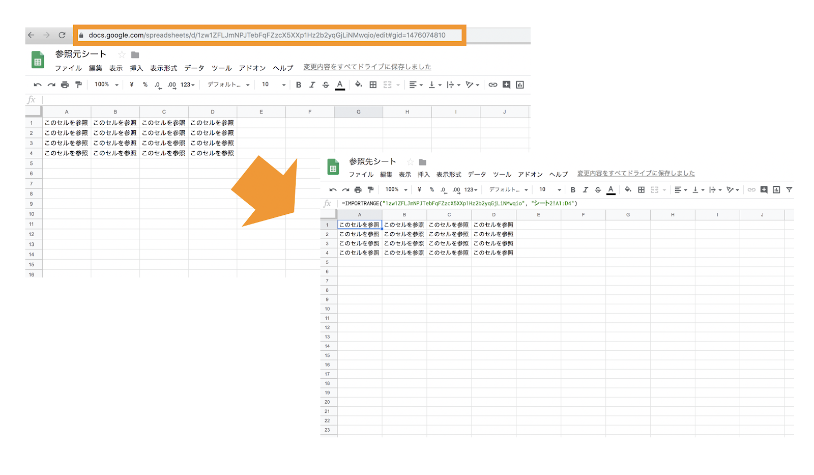
To summarize, if you type the following formula on the cell of the spreadsheet you want to quote, the data will be reflected instantly.
How to: Calculate Values from Another Spreadsheet
For example, you may want to calculate values from another spreadsheet and reflect them in the other spreadsheet.
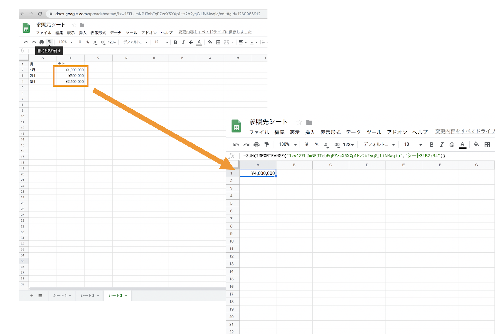
Case 1: Sum Using the SUM Function
Let’s assume that you want the sum of the amounts on another spreadsheet to be referenced by the other spreadsheet.
You can use the following formulas in the SUM function:.
Of course, it can be expressed by functions other than the SUM function. AVERAGE, SUMIF or COUNTIF can be set.
Case 2: Using the VLOOKUP Function
You can also use the VLOOKUP function.
For example, you can specify the product ID of the referencing sheet and display the product name.
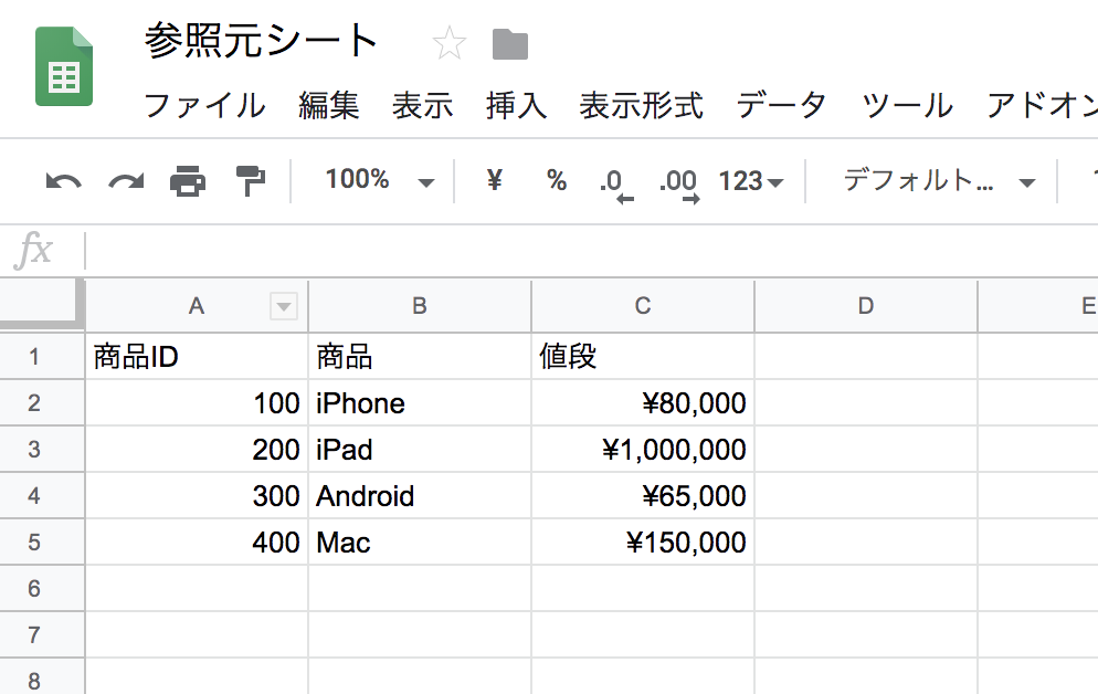
If you try to quote the item with item ID 100, the formula will be as follows.
The range of this value is A1: C5.
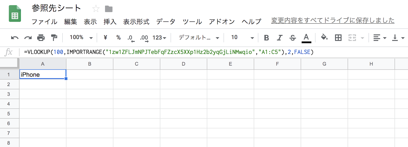
As shown above, “iPhone” was successfully displayed.
A description of the VLOOKUP function is beyond the scope of this article.
Reference values from another sheet in the same spreadsheet
If the spreadsheet is the same, but the sheets are different, enter the following formula:.
For example, if the sheet name you want to refer to is “Database B” and the cell you want to refer to is “A5”:.
This is very easy.
And finally,
I end my article on references from another spreadsheet that I have a chance to use.
Spreadsheets are a very deep and easy-to-use service, so you can see a lot of options for work efficiency and problem solving.
Of course, you don’t have to memorize functions, so please google it!